Rabbits and foxes

Building the model

Let the constant \(a\) as being the rate of reproduction of the rabbits: how many baby rabbits an adult rabbit has per month. So, the rabbits grow according to

(1)\[\frac{dR}{dt} = a R\]

This equation denotes the rate of change of \(R\) over time. the top part of the fraction \(dR\) denotes the change in rabbits, \(R\), and the bottom part, \(dt\), denotes the change in time, \(t\). The rabbits grow proportionally to the number of rabbits.

Let’s add a term to describe how foxes eat rabbits. The rate of change for rabbits now becomes

(2)\[\frac{dR}{dt} = a R - b R F\]

Similarly, we can write the rate of change of foxes as

(3)\[\frac{dF}{dt} = \underbrace{c R F}_{\mbox{F} + \mbox{R} \xrightarrow{c} 2 \mbox{F}} - \underbrace{d R}_{\mbox{R} \xrightarrow{d} 2 \mbox{R}}\]

Notice that we have a different rate parameter for the death of rabbits (\(b\)) than for the birth of foxes (\(c\)). This is because it takes more than one rabbit to feed a fox and we set the parameters so that \(c<b\).

A mathematical model like this is not to be entirely realistic. Rather, it tries to capture the essence of the problem. We want to imagine a big grassy meadow, where the more rabbits there are, the faster the rabbit population grows and the more foxes there are the faster the rabbits are eaten. We will try to understand this abstract problem first, before we make any claims about what happens to real rabbits and real foxes.

Simulating the model

We can use Python to run a numerical simulation of the model.

# Import the libraries we use
import numpy as np
import matplotlib.pyplot as plt
import matplotlib
from pylab import rcParams
matplotlib.font_manager.FontProperties(family='Helvetica',size=11)
rcParams['figure.figsize'] = 14/2.54, 10/2.54
from scipy import integrate

We start by defining the model. This code creates a function which we can use to simulate differential equations (2) and (3).

# Differential equation
def dXdt(X, t=0):
    # Growth rate of fox and rabbit populations.
    return np.array([ a*X[0]        - b*X[0]*X[1] ,      #Rabbits X[0] is R
                      c*X[0]*X[1]   - d*X[1]])           #Foxes X[1] is F

Next we define the parameter values. You can change these to see how changes to the paramaters leads to changes in the outcome of the model.

# Parameter values
a = 5
b = 1
c = 0.15
d = 1

Now we solve the equations numerically

t = np.linspace(0, 20,  1000)               # time
X0 = np.array([10, 2])                     # initially 10 rabbits and 2 foxes
X = integrate.odeint(dXdt, X0, t)
R, F = X.T

fig,ax=plt.subplots(num=1)
ax.plot(t, R, '-',color='k', label='Rabbits (R)')
ax.plot(t, F  , '--',color='k', label='Foxes (F)')
ax.legend(loc='best')
ax.set_xlabel('Time: t')
ax.set_ylabel('Population')
ax.spines['top'].set_visible(False)
ax.spines['right'].set_visible(False)
ax.set_xticks(np.arange(0,12,step=1))
ax.set_yticks(np.arange(0,50,step=10))
ax.set_xlim(0,12)
ax.set_ylim(0,25)
plt.show()

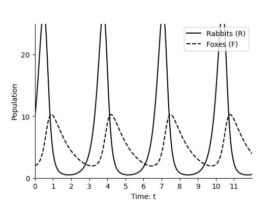
First the rabbit populations grow, because there are only two foxes. But this leads to an increase in foxes. Once the population of foxes is sufficiently large, they then start reducing rabbit populations and they die out. Then, when there are few rabbits left, the foxes start to die out too, allowing the rabbit population to grow again.

Visualising the cycle

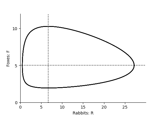
In the figure above, we show how foxes and rabbits change over time. We can also plot how they change relative to each other (a so called phase plane). For the numerical simulations we do this as follows:

def plotPhasePlane(ax,R,F):
    ax.plot(R, F, '-',color='k')
    ax.set_xlabel('Rabbits: R')
    ax.set_ylabel('Foxes: F')
    ax.spines['top'].set_visible(False)
    ax.spines['right'].set_visible(False)
    ax.set_xticks(np.arange(0,30,step=5))
    ax.set_yticks(np.arange(0,20,step=5))
    ax.set_ylim(0,12)
    ax.set_xlim(0,30)


fig,ax=plt.subplots(num=1)
plotPhasePlane(ax,R,F)
plt.show()

Finding the equilibrium

In order to better understand this cycle we look at the equilibria (the steady states) where the rate at which rabbits are born equals the rate at which they die. We can find the rabbit equilibtirum by solving

\[\frac{dR}{dt} = a R - b R F =0\]

i.e. the number of rabbits does not change over time. This occurs either when \(R=0\) (all the rabbits are dead) or when \(F=a/b\) (when the number of foxes is equal to the birth rate of rabbits divided by the rate at which foxes eat rabbits).

Similarly, we can find the fox equilibtirum by solving

\[\frac{dF}{dt} = c R F - d F =0\]

i.e. the number of foxes does not change over time. This occurs either when \(F=0\) (all the foxes are dead) or when \(R=d/c\) (when the number of rabbits is equal to the death rate of foxes divided by the rate at which foxes grow after eating rabbits).

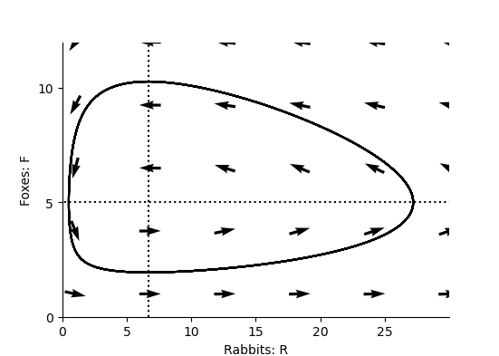
We can now plot these equilibrium on the phase plane

fig,ax=plt.subplots(num=1)
#Plot the rabbit equilibrium
ax.plot([-100,100],[a/b,a/b],linestyle=':',color='k')
#Plot the fox equilibrium
ax.plot([d/c,d/c],[-100,100],linestyle=':',color='k')
plotPhasePlane(ax,R,F)

We can draw arrows to indicate the direction of change. To do this, we evaluate \(dR/dt\) and \(dF/dt\) for different values and plot them.

x = np.linspace(1, 30 ,6)
y = np.linspace(1, 12, 5)
X , Y  = np.meshgrid(x, y)
dX, dY = dXdt([X, Y])
#Make in to unit vectors.
M = np.hypot(dX,dY)
dX = dX/M
dY = dY/M

fig,ax=plt.subplots(num=1)
ax.quiver(X, Y, dX, dY, pivot='mid')
#Plot the rabbit equilibrium
ax.plot([-100,100],[a/b,a/b],linestyle=':',color='k')
#Plot the fox equilibrium
ax.plot([d/c,d/c],[-100,100],linestyle=':',color='k')
plotPhasePlane(ax,R,F)