ARMA model

The moving average

The code below simulates the moving average model.

import random
import numpy as np
import matplotlib.pyplot as plt
import matplotlib
from pylab import rcParams
matplotlib.font_manager.FontProperties(family='Helvetica',size=11)
rcParams['figure.figsize'] = 14/2.54, 14/2.54


def plotOverTime(ax, w):
    n=len(w)
    t=np.arange(n)
    ax.plot(t,w, '-',color='k')
    ax.set_xlabel('Time: t')
    ax.spines['top'].set_visible(False)
    ax.spines['right'].set_visible(False)
    ax.set_xticks(np.arange(0,n,step=n/5))
    ax.set_yticks(np.arange(-n,n+1,step=10))
    ax.set_xlim(0,n)
    ax.set_ylim(-2*np.sqrt(n),2*np.sqrt(n))


def MA(w0,steps,c_vals,sigma=1):
    # n step random walk
    w = w0
    w_k = np.zeros(steps)

    #The random values can be produced in advance
    e_k = np.random.normal(0, 1,steps)

    for k in range(steps):
        w_k[k]= w

        #Add the most recent value
        w = e_k[k]

        #Add the weighted average of older values
        for j,c in enumerate(c_vals):
            w += c*e_k[k-j-1]

    return w_k


fig,axs=plt.subplots(3,3)
steps=100
for axsr in axs:
    for j,ax in enumerate(axsr):
        w=MA(0,steps,[0.5])
        plotOverTime(ax, w)
        if j==0:
            ax.set_ylabel('Position: w')

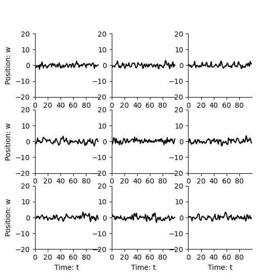
This process doesn’t move far from zero, because it has no “memory”.

Autogressive model

Here we plot the AR(1) model with :math;´a_1=-0.9´.

def AR(w0,steps,a_vals,sigma=1):
    # n step random walk

    n=len(w0)

    #Setup intial conditions
    w_k = np.zeros(steps)
    w_k[0:n-1] = w0

    #The random values can be produced in advance
    e_k = np.random.normal(0, 1,steps)

    for k in range(n,steps):

        #Add the noise
        w = e_k[k]

        #Add the weighted average of older values
        for j,a in enumerate(a_vals):
            w += -a*w_k[k-j-1]

        w_k[k]= w

    return w_k



fig,axs=plt.subplots(3,3)
steps=30
a_vals = [-0.9]
for axsr in axs:
    for j,ax in enumerate(axsr):
        w=AR([0],steps,a_vals)
        plotOverTime(ax, w)
        if j==0:
            ax.set_ylabel('Position: w')

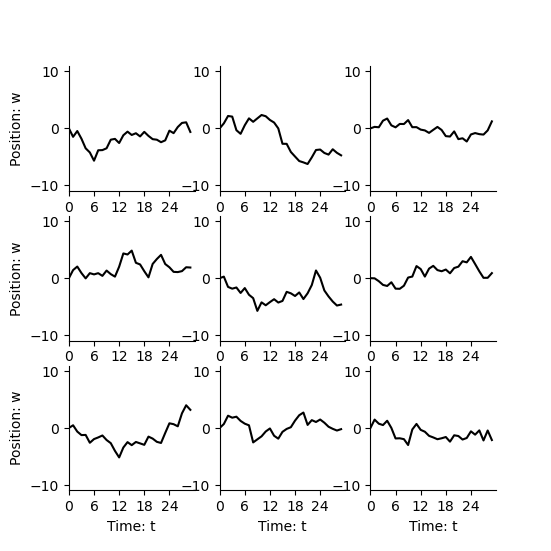
Now there is a longer memory. The process increases and decreases more slowly in comparison to the fluctuations caused by noise.

When we reduce :math;´a_1´ then the process moves more randomly, like the random walk.

fig,axs=plt.subplots(3,3)
steps=30
a_vals = [-0.1]
for axsr in axs:
    for j,ax in enumerate(axsr):
        w=AR([0],steps,a_vals)
        plotOverTime(ax, w)
        if j==0:
            ax.set_ylabel('Position: w')

If :math;´a_1´ is positive then the process oscilates backwards and forwards.

fig,axs=plt.subplots(3,3)
steps=30
a_vals = [0.9]
for axsr in axs:
    for j,ax in enumerate(axsr):
        w=AR([0],steps,a_vals)
        plotOverTime(ax, w)
        if j==0:
            ax.set_ylabel('Position: w')

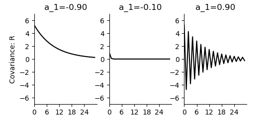
Theoretical covariance

The covariance functionfor AR(1) is calcuated as follows.

def R_theoretical(a_vals,maxtau,sigma=1):
    R = np.zeros(maxtau)
    for tau in range(maxtau):
        R[tau] = np.power(-a_vals[0],tau)* (np.power(sigma,2)/(1-np.power(a_vals[0],2)))

    return R

rcParams['figure.figsize'] = 14/2.54, 6/2.54

fig,axs=plt.subplots(1,3)
for i,avals in enumerate([[-0.9],[-0.1],[0.9]]):

    ax=axs[i]
    if (i==0):
        ax.set_ylabel('Covariance: R')
    txt='a_1=%.2f'%avals[0]
    ax.set_title(txt)
    R=R_theoretical(avals,maxtau=steps)
    plotOverTime(ax, R)
    ax.set_yticks(np.arange(-10,10,step=2))
    ax.set_ylim(-7,7)

plt.show()

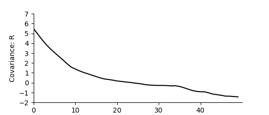
Empirical covariance

Fill in the code below to write a function yourself to calculate the empirical covariance.

Then use it to calculate the standard deviation over 1000 time steps of an AR(1) model with :math:´a_1=-0.9´.

def R_empirical(w,maxtau):

    steps=len(w)
    R = np.zeros(maxtau)
    for tau in range(maxtau):
        Rk = np.zeros(steps)
        for k,wk in enumerate(w):
            if k<steps-tau:
                Rk[k] =  w[k+tau]*w[k]

        R[tau] = np.sum(Rk)/(steps-tau)


    return R

fig,ax=plt.subplots(1)
ax.set_ylabel('Covariance: R')
a_vals = [-0.9]
steps=1000
w=AR([0],steps,a_vals)
R=R_empirical(w,maxtau=50)
plotOverTime(ax, R)
ax.set_yticks(np.arange(-10,10,step=1))
ax.set_ylim(-2,7)
plt.show()

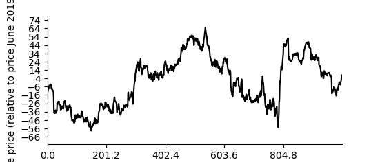
Share prices

Now let’s use your function to calulate a covariance function for H&M share prices. First lets load in and plot the data.

import pandas as pd

share_prices=pd.read_csv('../data/HandM.csv')
w = share_prices['Average price']
w=np.array(w.dropna())
fig,ax=plt.subplots(1)

w=w-np.mean(w)
plotOverTime(ax, w)
ax.set_ylabel('Share price (relative to price June 2019): w')
ax.set_ylim(-75,75)
plt.show()

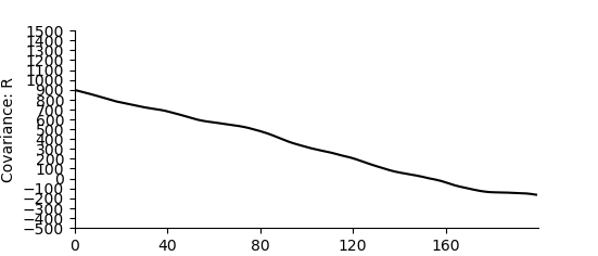
Share prices

Now plot the correlation as a function

fig,ax=plt.subplots(1)
R=R_empirical(w,maxtau=200)
plotOverTime(ax, R)
ax.set_yticks(np.arange(-600,1600,step=100))
ax.set_ylim(-500,1500)
ax.set_ylabel('Covariance: R')

Text(15.369860017497809, 0.5, 'Covariance: R')