Two variable model

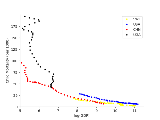
Plotting the data

We now make a Gapminder style plot of the data.

#Import libraries
#Plotting
import matplotlib as mpl
import matplotlib.pyplot as plt
import pandas as pd
import numpy as np

#Import machine learning tools (for linear regression)
import sklearn.linear_model as skl_lm
import itertools
import math

df = pd.read_csv('../data/CM_GDP.csv')

countries=['SWE','USA','CHN','UGA']
country_colour_dict= {
  "USA": "blue",
  "CHN": "red",
  "SWE": "yellow",
  "UGA": "black",
  "AFG": "green"
}

fig,ax=plt.subplots(num=1)
for country in countries:
    df_country=df.loc[df['Country'] == country]
    ax.plot(df_country['GDP'], df_country['Child Mortality'],linestyle='none', markersize=3, color =country_colour_dict[country],  marker='o',label=country)

ax.legend()
ax.set_xticks(np.arange(5,12,step=1))
ax.set_yticks(np.arange(0,200,step=25))
ax.set_ylabel('Child Mortality (per 1000)')
ax.set_xlabel('log(GDP)')
ax.spines['top'].set_visible(False)
ax.spines['right'].set_visible(False)
ax.set_ylim(0,201)
ax.set_xlim(5,11.5)

(5.0, 11.5)

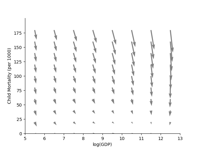
Fitting a model

Now we fit a linear regression model where child mortality and GDP can influence each other. We assume that

\[\begin{split} \begin{aligned} y_C(k) & = C(k+1) - C(k) = a_C + b_{C0} C(k) + b_{C1} C(k)^2 & \\ & + b_{C2} C(k)^3 + b_{C3} G(k) + b_{C4} G(k)^2 + b_{C5} C(k) G(k) + \epsilon_C(k)& \\ & , \qquad \epsilon_C(k) \sim \mathcal{N}(0, \sigma_C^2) \end{aligned}\end{split}\]

and

\[\begin{split} \begin{aligned} y_G(k) & = G(k+1) - G(k) = a_G + b_{G0} C(k) + b_{G1} C(k)^2 & \\ & + b_{G2} C(k)^3 + b_{G3} G(k) + b_{G4} G(k)^2 + b_{G5} C(k) G(k) + \epsilon_G(k) & \\ & , \qquad \epsilon_G(k) \sim \mathcal{N}(0, \sigma_G^2) \end{aligned}\end{split}\]

describes the interaction and fit the model below. We fit the model then plot the vector field it creates.

df['C2'] = df['Child Mortality']**2
df['C3'] = df['Child Mortality']**3
df['G2'] = df['GDP']**2
df['CG'] = df['GDP']*df['Child Mortality']
X_train = df[['Child Mortality','C2','C3','GDP','G2','CG']]
y_train = df['Diff CM']
model = skl_lm.LinearRegression(fit_intercept=True)
model.fit(X_train, y_train)
# Print the coefficients
print('The coefficients are:', model.coef_)
print('The offset is: {model.intercept_:.3f}')
G,C = np.meshgrid(np.arange(5.5, 13, step=1),np.arange(0, 200, step=20))
b = model.coef_
a =model.intercept_
dC = a + b[0] * C + b[1]*C**2 + b[2]*C**3 + b[3]*G + b[4]*G**2 + b[5]*C*G


X_train = df[['Child Mortality','C2','C3','GDP','G2','CG']]
y_train = df['Diff GDP']
model = skl_lm.LinearRegression(fit_intercept=True)
model.fit(X_train, y_train)
# Print the coefficients
print('The coefficients are:', model.coef_)
print('The offset is: {model.intercept_:.3f}')
bG = model.coef_
aG =model.intercept_
dG = aG + bG[0] * C + bG[1]*C**2 + bG[2]*C**3 + bG[3]*G + bG[4]*G**2 + bG[5]*C*G


fig,ax=plt.subplots(num=1)
ax.quiver(G,C,dG*20,dC,color='grey')
ax.set_xticks(np.arange(5,13.5,step=1))
ax.set_yticks(np.arange(0,200,step=25))
ax.set_ylabel('Child Mortality (per 1000)')
ax.set_xlabel('log(GDP)')
ax.spines['top'].set_visible(False)
ax.spines['right'].set_visible(False)
ax.set_ylim(0,201)
ax.set_xlim(5,13)
plt.show()

The coefficients are: [ 1.46411726e-02 -2.38007308e-05  2.05646960e-07  1.77883326e+00
 -8.79490494e-02 -5.84214256e-03]
The offset is: {model.intercept_:.3f}
The coefficients are: [-9.97793571e-04  4.01217410e-06 -6.50712348e-09  4.55148930e-02
 -3.13345168e-03  7.30278312e-05]
The offset is: {model.intercept_:.3f}

We will simulate this model as one of the exercises on the next page.