Do it yourself

Fitting a single variable model to GDP

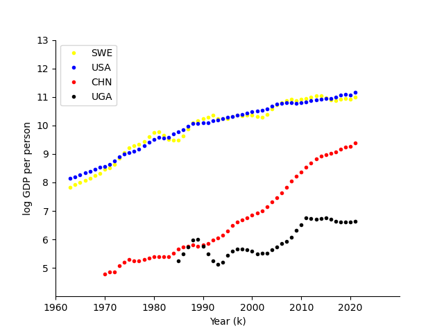
The plot below should show change in GDP for the four countries. The code below is wrong. Complete it by filling in the correct code below.

#Import libraries
#Plotting
import matplotlib.pyplot as plt
import pandas as pd
import numpy as np
import sklearn.linear_model as skl_lm

df = pd.read_csv('../data/CM_GDP.csv')

countries=['SWE','USA','CHN','UGA']
country_colour_dict= {
  "USA": "blue",
  "CHN": "red",
  "SWE": "yellow",
  "UGA": "black",
  "AFG": "green"
}

fig,ax=plt.subplots(num=1)
for country in countries:
    df_country=df.loc[df['Country'] == country]

    years=np.array(df_country['Year']).astype('int32')
    ax.plot(years,df_country['GDP'],linestyle='none', color =country_colour_dict[country], markersize=3, marker='o',label=country)
ax.legend()
ax.set_xticks(np.arange(1960,2030,step=10))
ax.set_yticks(np.arange(5,14,step=1))
ax.set_ylabel('log GDP per person')
ax.set_xlabel('Year (k)')
ax.spines['top'].set_visible(False)
ax.spines['right'].set_visible(False)
ax.set_xlim(1960,2030)
ax.set_ylim(4,13)

plt.show()

Single variable

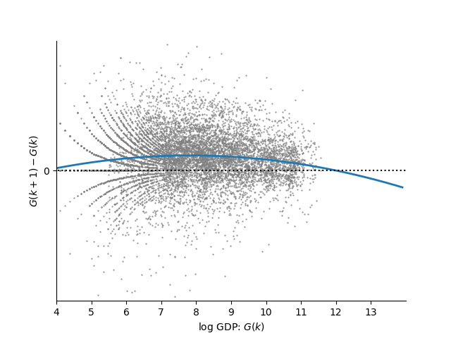
Fit a linear regression model

\[y(k) = G(k+1) - G(k) = a + b_0 G(k) + b_1 G(k)^2 + \epsilon, \qquad \epsilon \sim \mathcal{N}(0, \sigma^2)\]

to describe the change in log(GDP) from one year to the next. Again, fill in the blanks.

#Create the variables
df['G2'] = df['GDP']**2
#Set up the model
X_train = df[['GDP','G2']]
y_train = df['Diff GDP']
#Fit the model
model = skl_lm.LinearRegression(fit_intercept=True)
model.fit(X_train, y_train)
# Print the coefficients
print('The coefficients are:', model.coef_)
print(f'The offset is: {model.intercept_:.3f}')
b = model.coef_
a=model.intercept_

G = np.arange(0,14,0.1)
dG = a + b[0] * G + b[1]*G**2

The coefficients are: [ 0.05212442 -0.00332776]
The offset is: -0.146

Make a plot of the change in GDP as a function of GDP.

fig,ax=plt.subplots(num=1)
ax.plot(df['GDP'],df['Diff GDP'],linestyle='none', markersize=1,color='grey',marker='.')
ax.plot(G,dG,linewidth=2)
ax.plot([0 ,200],[0, 0],linestyle=':',color='black')
ax.set_yticks(np.arange(-5,0.5,step=1))
ax.set_xticks(np.arange(4,14,step=1))
ax.set_ylabel('$G(k+1)-G(k)$')
ax.set_xlabel('log GDP: $G(k)$')
ax.spines['top'].set_visible(False)
ax.spines['right'].set_visible(False)
ax.set_xlim(4,14)
ax.set_ylim(-0.5,0.5)
plt.show()

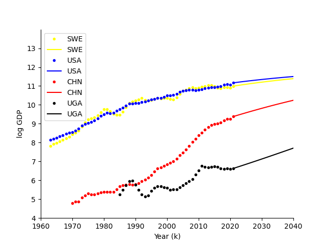
Predict future evoltion of GDP

fig,ax=plt.subplots(num=1)
for country in countries:
    df_country=df.loc[df['Country'] == country]

    years=np.array(df_country['Year']).astype('int32')
    ax.plot(years,df_country['GDP'],linestyle='none', color =country_colour_dict[country], markersize=3, marker='o',label=country)

    numyears=20
    future_GDP=np.zeros(numyears)
    future_GDP[0]=df_country['GDP'][-1:]


    for t in range(numyears-1):
        future_GDP[t+1]=future_GDP[t]+ a + b[0] * future_GDP[t] + b[1]*future_GDP[t]**2

    ax.plot(int(df_country['Year'][-1:])+np.arange(numyears),future_GDP, color =country_colour_dict[country],linestyle='-',label=country)
ax.legend()
ax.set_xticks(np.arange(1960,2045,step=10))
ax.set_yticks(np.arange(4,14,step=1))
ax.set_ylabel('log GDP')
ax.set_xlabel('Year (k)')
ax.spines['top'].set_visible(False)
ax.spines['right'].set_visible(False)
ax.set_xlim(1960,2040)
ax.set_ylim(4,14)
plt.show()

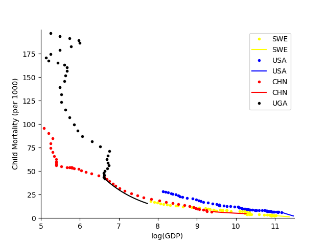
Two variables

Fill in the code below to simulate the model we fitted on page `twovariable`_ to make predictions of how child mortality and GDP will chnage over the next 30 years.

The co-efficients in your simulated model must be the same as the ones you found when fitting the model.

a =-8.858454419403133
b = np.array([ 1.46411726e-02, -2.38007308e-05,  2.05646960e-07,  1.77883326e+00,
       -8.79490494e-02, -5.84214256e-03])
aG=  -0.09681972964030267
bG = np.array([-9.97793571e-04,  4.01217410e-06, -6.50712348e-09,  4.55148930e-02,
       -3.13345168e-03,  7.30278312e-05])



fig,ax=plt.subplots(num=1)
for country in countries:
    df_country=df.loc[df['Country'] == country]
    ax.plot(df_country['GDP'], df_country['Child Mortality'],linestyle='none', markersize=3, color =country_colour_dict[country],  marker='o',label=country)

    numyears=20
    future_CM=np.zeros(numyears)
    future_CM[0]=df_country['Child Mortality'][-1:]
    future_GDP=np.zeros(numyears)
    future_GDP[0]=df_country['GDP'][-1:]

    ax.legend()

    for t in range(numyears-1):
        future_CM[t+1]=future_CM[t]+ a + b[0] * future_CM[t] + b[1]*future_CM[t]**2 + b[2]*future_CM[t]**3  + b[3]*future_GDP[t] + b[4]*future_GDP[t]**2 + b[5]*future_CM[t]*future_GDP[t]
        future_GDP[t+1]=future_GDP[t]+ aG + bG[0] * future_CM[t] + bG[1]*future_CM[t]**2 + bG[2]*future_CM[t]**3 + bG[3]*future_GDP[t] + bG[4]*future_GDP[t]**2 + bG[5]*future_CM[t]*future_GDP[t]

    ax.plot(future_GDP,future_CM, color =country_colour_dict[country],linestyle='-',label=country)

ax.set_xticks(np.arange(5,12,step=1))
ax.set_yticks(np.arange(0,200,step=25))
ax.set_ylabel('Child Mortality (per 1000)')
ax.set_xlabel('log(GDP)')
ax.spines['top'].set_visible(False)
ax.spines['right'].set_visible(False)
ax.set_ylim(0,201)
ax.set_xlim(5,11.5)

(5.0, 11.5)