Single variable model

Plotting the data

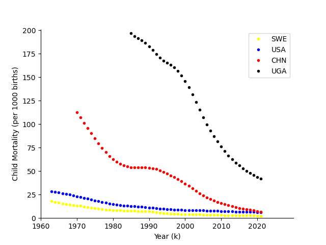
We now plot how child mortality has changed in four countries (Sweden, USA, Uganda and China).

In order look at other countries you can find their codes by looking here here and clicking on the country and then clicking on (i) to see country code.

#Import libraries
#Plotting
import matplotlib as mpl
import matplotlib.pyplot as plt
import pandas as pd
import numpy as np

#Import machine learning tools (for linear regression)
import sklearn.linear_model as skl_lm
import itertools
import math

df = pd.read_csv('../data/CM_GDP.csv')

countries=['SWE','USA','CHN','UGA']
country_colour_dict= {
  "USA": "blue",
  "CHN": "red",
  "SWE": "yellow",
  "UGA": "black",
  "AFG": "green"
}

fig,ax=plt.subplots(num=1)
for country in countries:
    df_country=df.loc[df['Country'] == country]

    years=np.array(df_country['Year']).astype('int32')
    ax.plot(years,df_country['Child Mortality'],linestyle='none', color =country_colour_dict[country], markersize=3, marker='o',label=country)
ax.legend()
ax.set_xticks(np.arange(1960,2030,step=10))
ax.set_yticks(np.arange(0,225,step=25))
ax.set_ylabel('Child Mortality (per 1000 births)')
ax.set_xlabel('Year (k)')
ax.spines['top'].set_visible(False)
ax.spines['right'].set_visible(False)
ax.set_xlim(1960,2030)
ax.set_ylim(0,201)

plt.show()

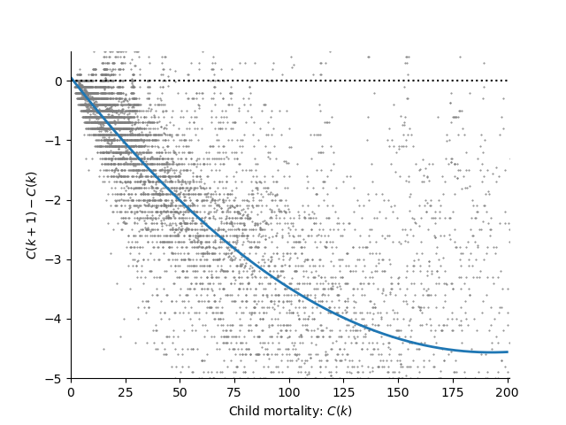
Fitting a model to child mortality

Now we fit a linear regression model

\[y(k) = C(k+1) - C(k) = a + b_0 C(k) + b_1 C(k)^2 + b_2 C(k)^3 + \epsilon, \qquad \epsilon \sim \mathcal{N}(0, \sigma^2)\]

to describe the change in child mortality from one year to the next.

To do this we use scikitlearn library in Python.

#Create the variables
df['C2'] = df['Child Mortality']**2
df['C3'] = df['Child Mortality']**3
X_train = df[['Child Mortality','C2','C3']]
y_train = df['Diff CM']
model = skl_lm.LinearRegression(fit_intercept=True)
model.fit(X_train, y_train)
# Print the coefficients
print('The coefficients are:', model.coef_)
print(f'The intercept is: {model.intercept_:.3f}')
b = model.coef_
a=model.intercept_

The coefficients are: [-4.72477545e-02  1.17046559e-04  1.90575426e-08]
The intercept is: 0.057

We can now plot the fitted model on the same plot as the data.

C = np.arange(0,200,0.1)
dC = a + b[0] * C + b[1]*C**2 + b[2]*C**3

#Make the plot
fig,ax=plt.subplots(num=1)
ax.plot(df['Child Mortality'],df['Diff CM'],linestyle='none', markersize=1,color='grey',marker='.')
ax.plot(C,dC,linewidth=2)
ax.plot([0 ,200],[0, 0],linestyle=':',color='black')
ax.set_yticks(np.arange(-5,0.5,step=1))
ax.set_xticks(np.arange(0,225,step=25))
ax.set_ylabel('$C(k+1)-C(k)$')
ax.set_xlabel('Child mortality: $C(k)$')
ax.spines['top'].set_visible(False)
ax.spines['right'].set_visible(False)
ax.set_xlim(0,201)
ax.set_ylim(-5,0.5)
plt.show()

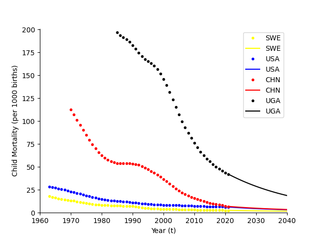
Predict future evoltion of child mortality

fig,ax=plt.subplots(num=1)
for country in countries:
    df_country=df.loc[df['Country'] == country]

    years=np.array(df_country['Year']).astype('int32')
    ax.plot(years,df_country['Child Mortality'],linestyle='none', color =country_colour_dict[country], markersize=3, marker='o',label=country)

    numyears=20
    future_CM=np.zeros(numyears)
    future_CM[0]=df_country['Child Mortality'][-1:]


    for t in range(numyears-1):
        future_CM[t+1]=future_CM[t]+ a + b[0] * future_CM[t] + b[1]*future_CM[t]**2 + b[2]*future_CM[t]**3

    ax.plot(int(df_country['Year'][-1:])+np.arange(numyears),future_CM, color =country_colour_dict[country],linestyle='-',label=country)
ax.legend()
ax.set_xticks(np.arange(1960,2045,step=10))
ax.set_yticks(np.arange(0,225,step=25))
ax.set_ylabel('Child Mortality (per 1000 births)')
ax.set_xlabel('Year (t)')
ax.spines['top'].set_visible(False)
ax.spines['right'].set_visible(False)
ax.set_xlim(1960,2040)
ax.set_ylim(0,201)
plt.show()